Using the MHW-CI database to plot
using_mhw_database.Rmd
library(magrittr)
library(mhwci)
library(ggplot2)
require(duckdb)
#> Loading required package: duckdb
#> Loading required package: DBI
This shows some basic commands to connect to the MHW-CI database, summarize data and plot.
If you are developing this package, editing scripts or adding
packages, then run this in the console prior to this script:
devtools::load_all()
This package requires a database file that stores all the data. You have to create a database ‘connection’ first
You can type the filename in a variable
# read from the environment
db_file <- "db/mhwci_v3.db"
or you can set the path to the database file in an
.Renviron file like this
MHWDBFILE=/Users/billspat/Code/SpaCELab/marine_heatwave_work/mhwci/db/mhwci_v3.db
Note that MHWDBFILE must be the full path to the database file. If
you do set it in the .Renviron file, then you can use this
function:
# read from the environment
db_file <- mhwci::get_dbfile()
#> Warning in mhwci::get_dbfile(): default dbfile set to
#> /Users/billspat/Code/SpaCELab/marine_heatwave_work/mhwci/db/mhwci_v4.db
Then you need to create a connection object:
db<- mhwci::mhw_connect(db_file)
print(db)
#> <duckdb_connection 3eee0 driver=<duckdb_driver dbdir='/Users/billspat/Code/SpaCELab/marine_heatwave_work/mhwci/db/mhwci_v4.db' read_only=FALSE bigint=numeric>>
This isn’t actually the database, just a connection to it required for all database functions.
Now you could list the tables in the database:
print(duckdb::dbListTables(db))
#>  [1] "all_lat_lon"
#>  [2] "arise10_decade_metrics"
#>  [3] "arise10_metrics"
#>  [4] "arise15_decade_metrics"
#>  [5] "arise15_metrics"
#>  [6] "avg_duration_by_decade_arise10"
#>  [7] "avg_duration_by_decade_truncated_arise10"
#>  [8] "decades"
#>  [9] "ensembles"
#> [10] "historical"
#> [11] "lat_index"
#> [12] "lon_index"
#> [13] "ssp245_decade_metrics"
#> [14] "ssp245_metrics"
#> [15] "years"
The database has a table for each scenario, listed above, and a few
other support tables. This package has a quick function to look at the
first few rows of a table, similar to the Unix head
command.
mhwci::table_head(db,"ssp245_decade_metrics")
#>    mhw_onset  mhw_end mhw_dur    int_max   int_mean    int_var    int_cum xloc
#> 1   20630126 20630421      86 0.13075171 0.06153818 0.02267874   5.292284  278
#> 2   20640119 20640627     160 1.53004237 0.29500325 0.38347423  47.200520  278
#> 3   20640709 20650430     296 2.63857318 1.18621743 0.89053356 351.120359  278
#> 4   20661213 20661222      10 0.32314950 0.20344789 0.05978969   2.034479  278
#> 5   20670111 20670121      11 0.09851572 0.07938800 0.01561200   0.873268  278
#> 6   20621012 20621104      24 1.07918261 0.94141387 0.10156655  22.593933  278
#> 7   20611107 20620505     180 0.20390204 0.08334335 0.03855356  15.001804  278
#> 8   20660721 20670529     313 1.87266755 0.50421482 0.60072794 157.819240  278
#> 9   20670602 20670615      14 0.28487715 0.18350036 0.05155543   2.569005  278
#> 10  20680609 20690604     361 2.70109577 0.73765259 0.85981247 266.292584  278
#>    yloc ensemble scenario mhw_onset_date mhw_end_date      lat    lon
#> 1   173      010  SSP-245     2063-01-26   2063-04-21 72.09424 346.25
#> 2   173      010  SSP-245     2064-01-19   2064-06-27 72.09424 346.25
#> 3   173      010  SSP-245     2064-07-09   2065-04-30 72.09424 346.25
#> 4   173      010  SSP-245     2066-12-13   2066-12-22 72.09424 346.25
#> 5   173      010  SSP-245     2067-01-11   2067-01-21 72.09424 346.25
#> 6   174      010  SSP-245     2062-10-12   2062-11-04 73.03665 346.25
#> 7   175      010  SSP-245     2061-11-07   2062-05-05 73.97906 346.25
#> 8   175      010  SSP-245     2066-07-21   2067-05-29 73.97906 346.25
#> 9   175      010  SSP-245     2067-06-02   2067-06-15 73.97906 346.25
#> 10  175      010  SSP-245     2068-06-09   2069-06-04 73.97906 346.25
Calculating Metrics
Set the scenario table to use for this plot.
mhw_table <-"arise10_decade_metrics"This function queries this table for average durations by point and
decade into data frames with x, y and value, and then uses the
terra package to create the rasters of those decades in a
list. It also rotates the world plots so that the center is along the
prime meridian instead of the dateline.
raster_list <- durations_by_decade_raster(db, mhw_table)
print(raster_list)
#> class       : SpatRaster
#> dimensions  : 178, 288, 3  (nrow, ncol, nlyr)
#> resolution  : 1.25, 0.9424084  (x, y)
#> extent      : -180.625, 179.375, -78.2199, 89.5288  (xmin, xmax, ymin, ymax)
#> coord. ref. : WGS 84 / World Equidistant Cylindrical (EPSG:4087)
#> source(s)   : memory
#> names       :     2040,     2050,    2060
#> min values  :   5.0000,   5.0000,    5.00
#> max values  : 352.6837, 760.3404, 3040.25
Plot this list of rasters, setting the name of the metric (average duration) and the threshold of 1/2 year. Set the title to “” to not have a title.
plot_rasters_squish_outliers(raster_list, title = mhw_table,
                             subtitle = "average duration",
                             scale_label = "Average Duration, d",
                             )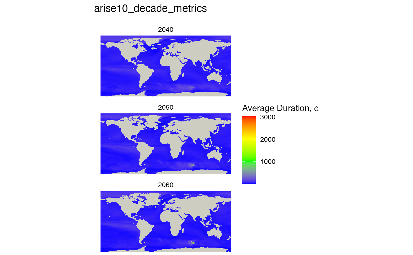
The reason there is no visible effect is because of the very long tail in the distribution.
# plot histogram of 3rd raster, 2060-

avg_dur_2060_69 <- na.omit(terra::values(raster_list[['2060']] ))

ggplot()+geom_histogram(aes(avg_dur_2060_69), bins=100)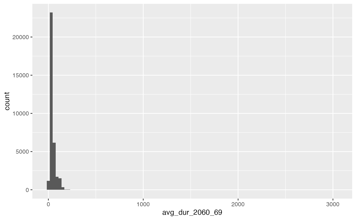
g<- ggplot()+geom_histogram(aes(na.omit(terra::values(raster_list[[3]]))), bins=100)Log Scale on X and Y
g + ggplot2::scale_x_log10() + ggplot2::scale_y_log10()
#> Warning in ggplot2::scale_y_log10(): log-10 transformation
#> introduced infinite values.
#> Warning: Removed 15 rows containing missing values or values outside the scale range
#> (`geom_bar()`).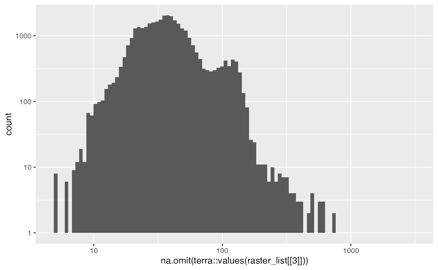
Plot duration other scenarios, set threshold
Combine the commands above to plot the other scenarios. This re-uses
the connection object db we created above. The
durations_by_decade_raster() creates the SQL and run is
against on the database
For plotting you can change the titles but also sets the
max_threshold_value to 1/2 year for this example. Note: * this
parameter used to be just threshold but now there is
max_threshold_value and min_threshold_value*
raster_list <- durations_by_decade_raster(db, mhw_table= "arise15_decade_metrics")
plot_rasters_squish_outliers(raster_list, title = "ARISE 1.5 Average Duration",
                             subtitle = "Threshold 1/2 year",
                             scale_label = "Mean Duration, d",
                             max_threshold_value = 365/2)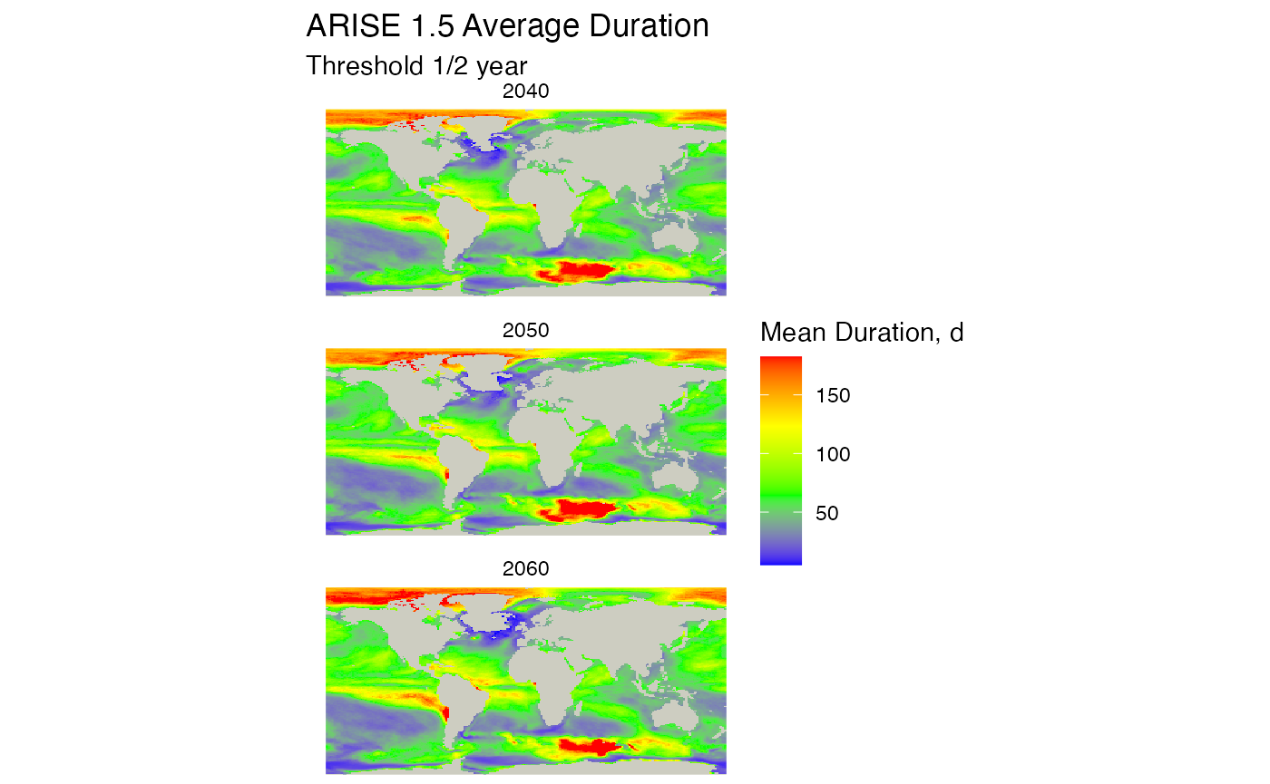
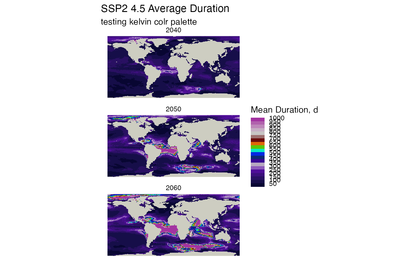
For this function, by default, the color scale is continuous. If you
send a break_width parameter it will make it discrete. and
also set a different color palette. See the reference documentation for
plot_rasters_squish_outliers() function for details
raster_list <- durations_by_decade_raster(db, mhw_table= "ssp245_decade_metrics")
grass_palette_name <- "kelvin"
plot_rasters_squish_outliers(raster_list, title = "SSP2 4.5 Average Duration",
                             subtitle = paste("testing", grass_palette_name, "colr palette"),
                             scale_label = "Mean Duration, d",
                             max_threshold_value = 1000,
                             break_width = 50,
                             palette_name = grass_palette_name
                             )
Plot other metrics and summaries
There are functions to summary any of the metrics with various statistics (mean, median, min, max, mode, etc)
Let’s take the average of the average intensity
# set the table
mhw_table <- "arise10_decade_metrics"
# select the metric or column in the table above
mhw_metric <- 'int_mean'
# select the summary function, must be one of the SQL functions, not an R function
sql_function <- 'avg'

#create the rasters for each decade for this metric, similar to duration but tis is a generic function
rm(raster_list)
raster_list <- metrics_by_decade_raster(db, mhw_table, mhw_metric = mhw_metric, sql_function = sql_function)

# plot, constructing the title from the variables we set above
# no threshold is set
plot_rasters_squish_outliers(raster_list,
                             title = paste(mhw_table, mhw_metric, sql_function),
                             scale_label = "avg intensity average, c" )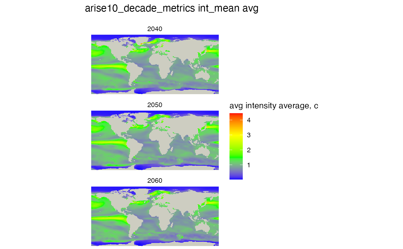
Filtering ensembles
If you use a special syntax, you can select which ensembles to use in
the summaries. The format is a string with list of ensembles and leading
zeros, like this "006,007,008" Ten has a leading zero to,
or "010" This is not a vector but a string! (for now). See
the code below
ensemble_list_string = "006,007,008"

#create the rasters for each decade for this metric, similar to duration but tis is a generic function
raster_list <- metrics_by_decade_raster(db, mhw_table, mhw_metric = mhw_metric, sql_function = sql_function,
                                        ensemble_list_string = ensemble_list_string )

# plot, constructing the title from the variables we set above
# no threshold is set
plot_rasters_squish_outliers(raster_list,
                             title = paste(mhw_table, mhw_metric, sql_function, " ensembles ", ensemble_list_string),
                             scale_label = "avg intensity average, c")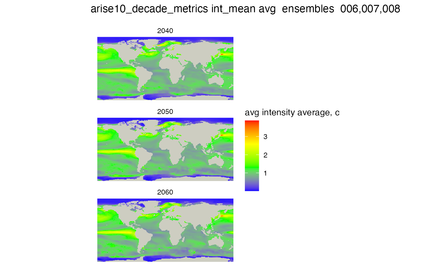
Using SQL directly
You can run SQL command to get data using the duckdb database engine, which is very fast.
This SQL averages duration for the specific table
# this is a function that creates a string of SQL with the table we want to use
sql_text<- avg_duration_by_decade_sql(mhw_table)
print(sql_text )
#> SELECT lat, lon, decades.decade, avg(mhw_dur) as avg_dur
#>   FROM arise10_decade_metrics, decades
#> WHERE ((mhw_onset_date >= decades.decade_start) AND (mhw_onset_date <= decades.decade_end))
#> GROUP BY lat, lon, decades.decade
Here is how you run a query:
# run this SQL using the `dbGetQuery` command.
duration_by_loc<- DBI::dbGetQuery(db, sql_text)
# show the first few rows
head(duration_by_loc)
#>         lat    lon decade  avg_dur
#> 1  56.07330 216.25   2050 41.71751
#> 2  87.17278 216.25   2050 69.37452
#> 3 -58.90052 217.50   2050 46.18519
#> 4  15.54974 217.50   2050 45.28395
#> 5  32.51309 217.50   2050 45.72065
#> 6  47.59162 217.50   2050 40.59551
Now close the connection used here, otherwise there may be errors (“could not set lock on file …”)
rm(duration_by_loc, raster_list)

dbDisconnect(db)